Metrics

All three metrics ask the same question of every sample: among its nearest neighbours in feature space, does it sit closer to samples that share its biology or to samples that share its confounder? They differ in how they turn that neighbourhood into a number.

RI counts typed neighbours inside a fixed k. MaRI keeps the fixed window but weights by distance. CRoMa drops the fixed window and compares the nearest SO and OS distances directly.

Neighbour types

Fix a sample with label \(\ell\) and confounder \(c\). Each of its neighbours falls into one of four types:

Type	Neighbour	Meaning
SO	same label, other confounder	The biological match. A robust model keeps these close.
OS	other label, same confounder	The confounder impostor. A shortcut-prone model keeps these close.
SS	same label, same confounder	Uninformative: biology and confounder agree.
OO	other label, other confounder	Uninformative: biology and confounder both differ.

Only SO and OS neighbours – the typed neighbours – carry evidence. Candidates sharing the query’s group_id – its independence group – are always excluded, so a model cannot score well by retrieving near-duplicates of the sample it is already looking at.

Note

A sample whose top-k contains no typed neighbour carries no evidence for RI and MaRI. The pooled score is still defined – it just silently rests on the subset of samples that do carry typed evidence. That subset, the support, is model-dependent: two models’ scores on the same cohort can summarize different sets of samples, which undermines a direct comparison between them. Always read the support fraction (1 - result.undefined_frac) alongside the score; a high RI resting on a thin support is not a strong result. CRoMa scores every sample instead, by searching outward until it finds typed neighbours.

Robustness Index

RI counts, and it counts at the dataset level. Within each sample’s top k, count the typed neighbours of each kind, \(n_{SO}(i)\) and \(n_{OS}(i)\); RI is the pooled share of all that typed evidence that is biological:

\[\mathrm{RI} = \frac{\sum_i n_{SO}(i)}{\sum_i \left( n_{SO}(i) + n_{OS}(i) \right)}\]

One number for the whole dataset, in \([0, 1]\): above 0.5 biology dominates the typed evidence, below it the confounder does. Two limitations follow from the form. Every counted neighbour weighs the same, whether adjacent to the sample or at the edge of the window, so RI cannot see how decisively biology wins – the gap MaRI closes. And because it pools raw counts, samples with richer typed neighbourhoods contribute more while samples with none contribute nothing at all – the support caveat in the note above.

k is not a free parameter. It is chosen from k_candidates as the value maximizing biological kNN balanced accuracy, so RI and MaRI always operate at the same k.

from croma import RI

ri = RI.compute(
    features, manifest,
    confounder_column="center",
    evaluation_design="paired_2x2",
    k_candidates=[5, 11, 21],
)
print(ri.value, ri.k, ri.undefined_frac)

Margin-aware Robustness Index

Two models can earn the same RI while one keeps its biological matches far closer than its impostors and the other barely separates them. MaRI recovers that difference by replacing each neighbour’s count of 1 with a weight \(\exp(-d / \tau)\), where \(d\) is its cosine distance: near neighbours dominate, distant ones fade. Everything else – the biological share, the pooling, the \([0, 1]\) range, the 0.5 neutral point – is as in RI, so RI is exactly MaRI with every weight set to 1.

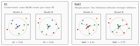
Same counts, different margins. The two neighbourhoods score identically under RI; weighting by distance separates them.

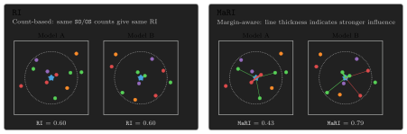
Same counts, different margins. The two neighbourhoods score identically under RI; weighting by distance separates them.

from croma import MaRI

mari = MaRI.compute(
    features, manifest,
    confounder_column="center",
    evaluation_design="paired_2x2",
    k_candidates=[5, 11, 21],
)
print(mari.value, mari.tau)

Choosing tau

tau sets how fast that weight decays, so it only means anything relative to the scale of the typed-neighbour distances. Far below that scale the score collapses onto the single nearest typed neighbour – winner-take-all, and noisy. Far above it every weight is \(\approx 1\) and MaRI degenerates back into count-based RI, losing the margin entirely.

That scale is a property of each embedding, not of the dataset: a tight representation’s typed neighbours sit much closer than a diffuse one’s. One fixed tau shared across models therefore sharpens the margin for some and flattens it for others – exactly the distortion MaRI exists to remove. So croma resolves it automatically, per model, as the median typed-neighbour cosine distance at the operating k, and reports the value used on result.tau. Leave it unset.

You can still pin tau – to reproduce a published number, say. croma warns if the pinned value sits more than a factor of 4 from the data’s typed-distance median; silence that with warn_tau=False. To inspect the recommendation without scoring, call recommend_tau().

Warning

Pinned tau values are comparable across models only if those models’ typed-neighbour distances share a scale. They generally do not.

Cross-confounder Robustness Margin

RI and MaRI share two structural limits: each compresses the whole dataset into one pooled number, and each rests on a model-dependent support – a sample with no typed neighbour inside k silently drops out of the pool. CRoMa removes both. It searches outward until it finds typed neighbours of both kinds, so it scores every sample, and each sample gets its own signed margin:

\[\mathrm{CRoMa}_i = \frac{d_{OS} - d_{SO}}{d_{OS} + d_{SO}}\]

where \(d_{SO}\) and \(d_{OS}\) are the mean cosine distances to the m nearest SO and OS neighbours. The result lies in \((-1, 1)\): positive is biology-dominant (the biological match is closer than the impostor), negative is confounder-dominant and fragile, and zero is an exactly contested boundary. The margin exists for every sample as long as the evaluation set holds at least m neighbours of each type – a property of the dataset, not the model, and satisfied by construction in the benchmark cohorts.

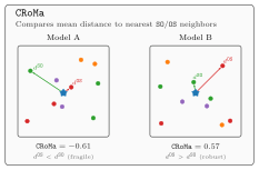
The same anchor under a fragile and a robust model. CRoMa is the normalized difference between the impostor distance and the biological-match distance.

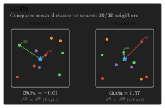
The same anchor under a fragile and a robust model. CRoMa is the normalized difference between the impostor distance and the biological-match distance.

from croma import CRoMa

croma = CRoMa.compute(
    features, manifest,
    confounder_column="center",
    evaluation_design="paired_2x2",
)
print(croma.value, croma.ltm_alpha, croma.f0)

Choosing m

m is the number of typed neighbours averaged per type. The default m=5 is the headline radius: m=1 is maximally sensitive to a single outlier neighbour, while m=5 is the smallest window in which no one neighbour exceeds 20% of the estimate, without leaving the local typed shell.

Model rankings and the biology-/confounder-dominant sign are near-invariant across m – Spearman \(\ge 0.98\) across the tile benchmarks – while m does move per-sample magnitudes and the tail statistics. Pass a list to sweep it in one pass:

results = CRoMa.compute(..., m=[1, 5, 10])   # -> dict[int, CRoMaResult]

The distribution, and its tail

Because every sample gets a margin, CRoMa produces something RI and MaRI cannot: a per-sample distribution over the full evaluation cohort. That distribution is the primary readout – it preserves the sample-level heterogeneity a pooled score compresses, and you can query it for whatever your deployment cares about (it is what the distribution explorer draws). value reports its middle; a model can look robust there while an identifiable slice of its samples is confounder-dominant, so every result also summarizes the fragile side from two angles:

• How bad – ltm_alpha, the lower-tail mean: the mean of the worst alpha fraction of samples (default 0.10). The severity of the failures.

• How common – f0, the confounder-dominant fraction \(F(0)\): the fraction of samples at or below zero. The prevalence of the failures.

Two models with the same median can differ sharply on both, and the lower tail is where deployment risk lives.

The confounder-dominant fraction

\(F(0)\) is the empirical CDF of the per-sample distribution at zero:

\[F(0) = \frac{\#\{i : \mathrm{CRoMa}_i \le 0\}}{\#\{i\}}\]

The inequality is closed: an exactly contested sample (\(\mathrm{CRoMa}_i = 0\), the impostor and the biological match equidistant) counts as confounder-dominant, because nothing about it says biology won. Under all each sample counts once; under paired_2x2 each subset occurrence counts once, so a sample scored in two subsets contributes twice. In the degenerate case of an evaluation set holding fewer than m typed neighbours of a kind, the unscorable samples are excluded from the denominator and reported by undefined_frac.

Read f0 as “how much of this model’s evidence is on the fragile side”, where value says where the middle of the distribution sits and ltm_alpha how bad the worst decile gets.